Analyze temporal signals with Satis
Introduction
Analyzing a temporal signal may seem a staightforward task. However, when you dive into this topic, several question may arise:
What is the mean value of my signal?
Does my signal capture all the frequencies of interest?
If this signal is the result of a simulation,
is my signal well discretized?
is my signal periodic?
what is the spectral power of my signal?
…
A canonical example of what we want to discuss here should be the following one:
 Mean pitfalls
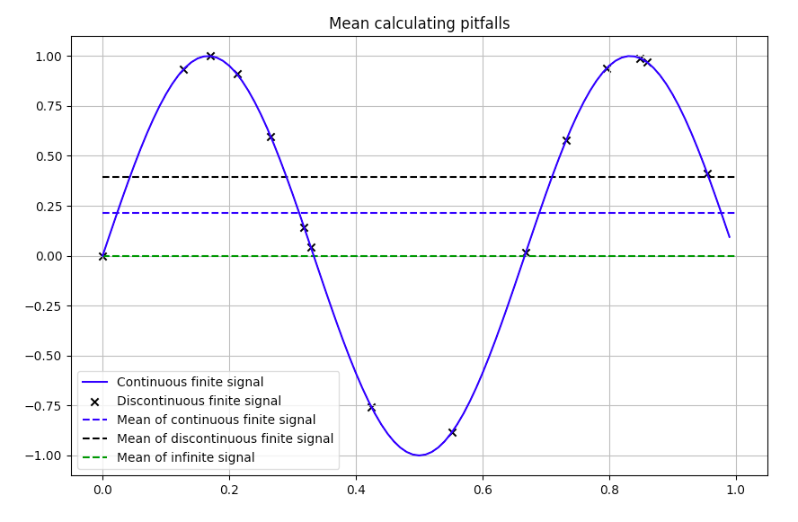
In this graph we have a sinus-shaped signal (blue curve). What is the mean value of this signal?
Well, it seems to be 0…
Ok, let’s keep this value in mind.
Imagine the signal is the result of a very complex numerical simulation and your time record makes the signal has been discretized at different time steps (black crosses). If we want to calculate the mean value of our signal, the ingenuous mind would calculate:
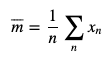 Classical mean
Doing so, one would get a mean value of approximatively 0.35.
Yes, but obviously the signal is poorly discretized!
Alright, if one had the same finite signal discretized at high frequency, averaging over the time record the value of the signal (to get close to the integral of the blue curve), one would have get a mean value of approx. 0.22.
…
The point of this example is to highlight the need to be aware of some traps in signal analysis. Cleaning up the signal before doing any calculation is a good practice. Hopefully, Satis provides a module named temporal_analysis_tool full of functions to help you avoiding these traps (see more information about Satis here.
Temporal_analysis_tool
Hereafter are detailed the functions you can find in the module temporal_analysis_tool plus how to use them. Generally, you will have to get your signal and put it in a time array and signal array:
record = numpy.genfromtxt("my_record.dat")
time = record[:,0]
signal = record[:,1]
resample_signal
Resample the initial signal at a constant time interval.
rescaled_time, rescaled_signal = resample_signal(time,
												 signal,
												 dtime=0.01)
NB: If a dtime is given, the interpolation is made to have a signal with a time interval of dtime. Else, the dt is the smallest time interval between two values of the signal.
calc_autocorrelation_time
Estimate the autocorrelation time at a given threshold.
The idea is: if you have a finite time record, you can always refine your signal, but at some point, you will not add any further information getting more points. This function returns the first time at which the signal is correlated under the threshold.
auto_time = calc_autocorrelation_time(time, signal, threshold=0.2)
sort_spectral_power
Determine the harmonic power contribution of the signal.
It calculates the Power Spectral Density (PSD) of the complete signal and of a downsampled version of the signal. The difference of the two PSD contains only harmonic components.
harmonic_power, total_power = sort_spectral_power(time, signal)
power_representative_frequency
Calculate the frequency that captures a level of spectral power.
It calculates the cumulative power spectral density and returns the frequency that reaches the threshold in percent of spectral power.
threshold_frequency = power_representative_frequency(time,
												     signal,
												     threshold=0.8)
duration_for_uncertainty
Give a suggestion of simulation duration to get an confidence interval range (around the mean) of the target value with a certain level of confidence.
This calculation is based on the Central Limit Theorem (CLT). It supposes several assumptions detailed in this notebook.
duration = duration_for_uncertainty(time,
									signal,
									target=10,
									confidence=0.95)
uncertainty_from_duration
Give a confidence interval range given the time step, the standard deviation, the duration and the level of confidence.
range = uncertainty_from_duration(dtime,
								  sigma,
								  duration,
								  confidence=0.95)
calculate_std
Give the standard deviation of a signal at a given frequency.
std = calculate_std(time, signal, frequency)
power_spectral_density
Automate the computation of the Power Spectral Density of a signal.
frequency, psd = power_spectral_density(time, signal)