Welcome to Satis
![]() logo
logo
Spectral Analysis for TImes Signals.
Satis is a python3 / scipy implementation of the Fourier Spectrums in Amplitude ans Power Spectral Density. It is particularly suited for CFD signals with the following characteristics:
Short sampling time,
Potentially short recording time,
Low signal-to-noise ratio,
Multiple measures available.
Installation
The package is available on PyPI so you can install it using pip:
pip install satis
How to use it
(my_env)rossi@pluto:~>satis


Usage: satis [OPTIONS] COMMAND [ARGS]...

  ---------------   SATIS  --------------------

  You are now using the Command line interface of Satis, a simple tool for
  spectral analysis optimized to signals from CFD, created at CERFACS
  (https://cerfacs.fr).

  This is a python package currently installed in your python environment.

Options:
  --help  Show this message and exit.

Commands:
  datasetforbeginners  Copy a set of signals to train using Satis.
  fourierconvergence   Plot discrete Fourier transform of the complete...
  fouriervariability   Plot the Fourier variability diagnostic results.
  psdconvergence       Plot the PSD convergence diagnostic results.
  psdvariability       Plot the spectral energy at the target frequency.
  time                 Plot the temporal signal and its time-average.
Several command lines are available on satis. You can display them running the command satis --help.
Dataset for beginners
satis datasetforbeginners
With this command , you can copy in your local directory a file my_first_dataset.dat to start using satis. It contains several signals of a CFD simulation. These signals have been recorded at different locations to create an average signal less sensitive to noise. For your first time with satis, we recommand to do the following diagnostics in the order with my_first_dataset.dat.
Time
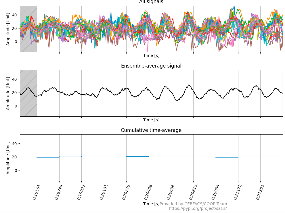
satis time my_first_dataset.dat
This diagnostic plots a time graph of your signals. This plot aims at showing you if the average signal is well converged or if there is a transient behavior. To delete a transient behavior, you can add at the end of the diagnostic command -t *starting_time* to declare the beginning of the converged behavior.
If a periodic pattern is visible, you should calculate its frequency and declare it with -f *calculated_frequency*
There is also a cumulative time-average. If this curve is not almost flat, you did probably not remove enough transient behavior.
 time diagnostic
Fourier variability
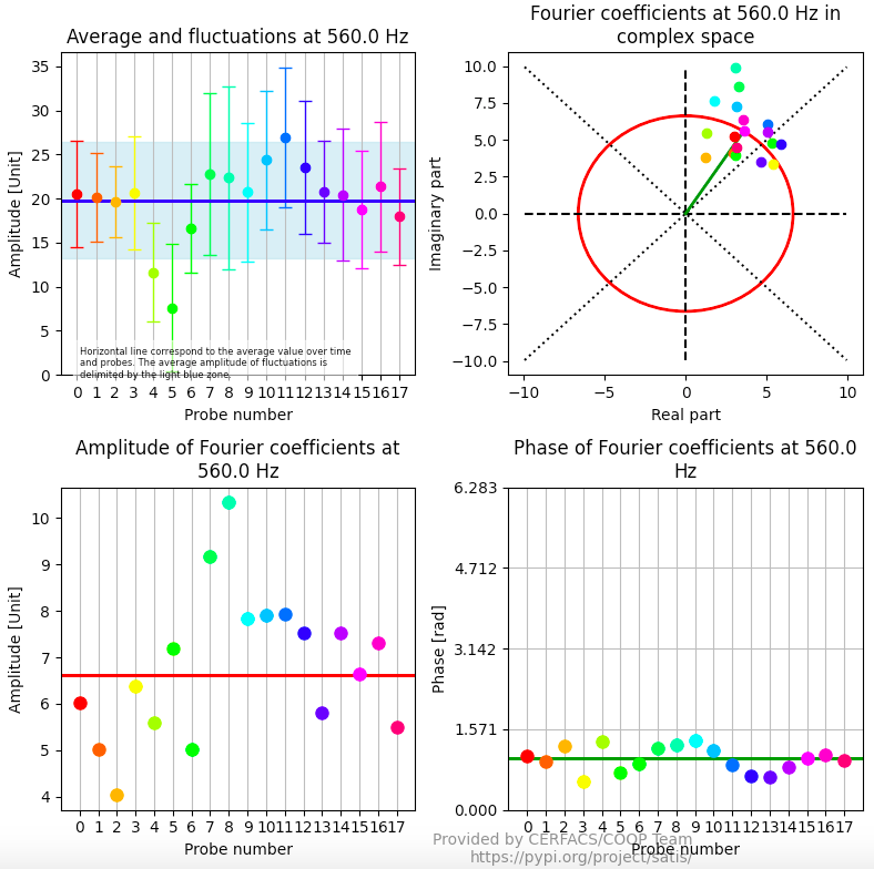
satis fouriervariability my_first_dataset.dat -t 0.201 -f 560
In this diagnostic, the Fourier coefficients of each signal at the specified frequency is plotted so that you can check the signals are equivalent. If a signal seems have different characteristics to the others, you should think about removing it. The average signal would be cleaner. To do so, declare the subset of signals you want to use with: --subset 1 3 14 ...
 fourier variability diagnostic
Fourier convergence
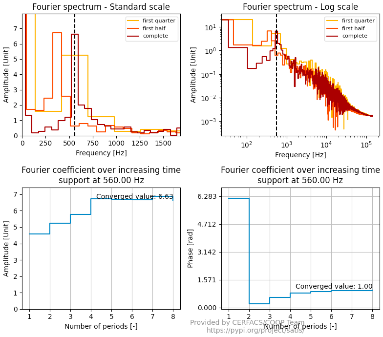
satis fourierconvergence my_first_dataset.dat -t 0.201 -f 560
Since this diagnostic is based on the average signal, the user should have checked beforehand that all input signals are equivalent thanks to the fouriervariability diagnostic.
The top plots show the amplitude of the Discrete Fourier Transform performed on the complete average signal, the last “half” of the signal and the last “quarter” of the signal.
The bottom plots show the convergence over increasing time of the amplitude and phase of the signal at the specified frequency.
 fourier convergence diagnostic
PSD variability
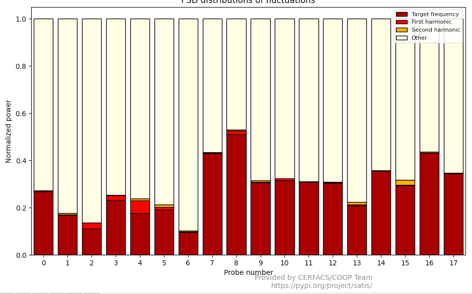
satis psdvariability my_first_dataset.dat -t 0.201 -f 560
This diagnostic shows the distribution of the spectral energy of fluctuations on the target frequency, its first and second harmonic and the rest of the frequencies. Note that this distribution is related to the fluctuations and that the time-average has been removed from the signal.
 psd variability diagnostic
PSD convergence
satis psdconvergence my_first_dataset.dat -t 0.201 -f 560
Just as the Fourier convergence, the PSD convergence diagnostic shows the Power Spectral Density obtained on the complete signal, the last half and the last quarter. The left uses a standard linear scale while the right plot shows the same result with log scales.
![psd convergence diagnostic]https://cerfacs.fr/coop/images/satis/psdconvergence.png)
Satis as a package
Of course, you can use satis in your own project importing it as a package:
import os
import glob
import satis
import matplotlib.pyplot as plt

*you awesome code*

time, signals = satis.read_signal('your_dataset.dat')
clean_time = satis.define_good_time_array(time, signals)
clean_signals = satis.interpolate_signals(time, signals, clean_time)
new_time, new_signals = satis.get_clean_signals(clean_time, signals,
												calculated_frequency)
plt.plot(new_time, new_signals)
fourier = satis.get_coeff_fourier(new_time, new_signals,
									calculated_frequency)

*your awesome code
Acknowledgements
This package is the result of work done at Cerfacs’s COOP Team. The contributors of this project are:
Franchine Ni
Antoine Dauptain
Tamon Nakano
Matthieu Rossi